Chaos Theory Facts For Kids

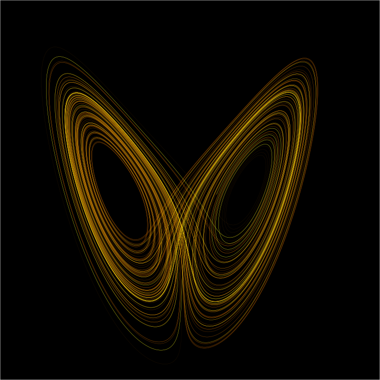
A plot of the 3D Lorenz attractor

An animation of a double-rod pendulum at an intermediate energy showing chaotic behavior. Starting the pendulum from a slightly different initial condition would result in a vastly different trajectory. The double-rod pendulum is one of the simplest dynamical systems with chaotic solutions.

The map defined by x → 4 x (1 – x) and y → (x + y) mod 1 displays sensitivity to initial x positions. Here, two series of x and y values diverge markedly over time from a tiny initial difference.

Lorenz equations used to generate plots for the y variable. The initial conditions for x and z were kept the same but those for y were changed between 1.001, 1.0001 and 1.00001. The values for ρ {displaystyle rho } , σ {displaystyle sigma } and β {displaystyle beta } were 45.91, 16 and 4 respectively. As can be seen from the graph, even the slightest difference in initial values causes significant changes after about 12 seconds of evolution in the three cases. This is an example of sensitive dependence on initial conditions.

Six iterations of a set of states [ x , y ] {displaystyle [x,y]} passed through the logistic map. The first iterate (blue) is the initial condition, which essentially forms a circle. Animation shows the first to the sixth iteration of the circular initial conditions. It can be seen that mixing occurs as we progress in iterations. The sixth iteration shows that the points are almost completely scattered in the phase space. Had we progressed further in iterations, the mixing would have been homogeneous and irreversible. The logistic map has equation x k + 1 = 4 x k ( 1 − x k ) {displaystyle x_{k+1}=4x_{k}(1-x_{k})} . To expand the state-space of the logistic map into two dimensions, a second state, y {displaystyle y} , was created as y k + 1 = x k + y k {displaystyle y_{k+1}=x_{k}+y_{k}} , if x k + y k < 1 {displaystyle x_{k}+y_{k}<1} and y k + 1 = x k + y k − 1 {displaystyle y_{k+1}=x_{k}+y_{k}-1} otherwise.

The map defined by x → 4 x (1 – x) and y → (x + y) mod 1 also displays topological mixing. Here, the blue region is transformed by the dynamics first to the purple region, then to the pink and red regions, and eventually to a cloud of vertical lines scattered across the space.

The Lorenz attractor displays chaotic behavior. These two plots demonstrate sensitive dependence on initial conditions within the region of phase space occupied by the attractor.

Coexisting chaotic and non-chaotic attractors within the generalized Lorenz model.[37][38][39] There are 128 orbits in different colors, beginning with different initial conditions for dimensionless time between 0.625 and 5 and a heating parameter r = 680. Chaotic orbits recurrently return close to the saddle point at the origin. Nonchaotic orbits eventually approach one of two stable critical points, as shown with large blue dots. Chaotic and nonchaotic orbits occupy different regions of attraction within the phase space.

Bifurcation diagram of the logistic map x → r x (1 – x). Each vertical slice shows the attractor for a specific value of r. The diagram displays period-doubling as r increases, eventually producing chaos. Darker points are visited more frequently.

A plot of the 3D Lorenz attractor

An animation of a double-rod pendulum at an intermediate energy showing chaotic behavior. Starting the pendulum from a slightly different initial condition would result in a vastly different trajectory. The double-rod pendulum is one of the simplest dynamical systems with chaotic solutions.

The map defined by x → 4 x (1 – x) and y → (x + y) mod 1 displays sensitivity to initial x positions. Here, two series of x and y values diverge markedly over time from a tiny initial difference.

Lorenz equations used to generate plots for the y variable. The initial conditions for x and z were kept the same but those for y were changed between 1.001, 1.0001 and 1.00001. The values for ρ {\displaystyle \rho } , σ {\displaystyle \sigma } and β {\displaystyle \beta } were 45.91, 16 and 4 respectively. As can be seen from the graph, even the slightest difference in initial values causes significant changes after about 12 seconds of evolution in the three cases. This is an example of sensitive dependence on initial conditions.

Six iterations of a set of states [ x , y ] {\displaystyle [x,y]} passed through the logistic map. The first iterate (blue) is the initial condition, which essentially forms a circle. Animation shows the first to the sixth iteration of the circular initial conditions. It can be seen that mixing occurs as we progress in iterations. The sixth iteration shows that the points are almost completely scattered in the phase space. Had we progressed further in iterations, the mixing would have been homogeneous and irreversible. The logistic map has equation x k + 1 = 4 x k ( 1 − x k ) {\displaystyle x_{k+1}=4x_{k}(1-x_{k})} . To expand the state-space of the logistic map into two dimensions, a second state, y {\displaystyle y} , was created as y k + 1 = x k + y k {\displaystyle y_{k+1}=x_{k}+y_{k}} , if x k + y k < 1 {\displaystyle x_{k}+y_{k}<1} and y k + 1 = x k + y k − 1 {\displaystyle y_{k+1}=x_{k}+y_{k}-1} otherwise.

The map defined by x → 4 x (1 – x) and y → (x + y) mod 1 also displays topological mixing. Here, the blue region is transformed by the dynamics first to the purple region, then to the pink and red regions, and eventually to a cloud of vertical lines scattered across the space.

The Lorenz attractor displays chaotic behavior. These two plots demonstrate sensitive dependence on initial conditions within the region of phase space occupied by the attractor.

Coexisting chaotic and non-chaotic attractors within the generalized Lorenz model.[37][38][39] There are 128 orbits in different colors, beginning with different initial conditions for dimensionless time between 0.625 and 5 and a heating parameter r = 680. Chaotic orbits recurrently return close to the saddle point at the origin. Nonchaotic orbits eventually approach one of two stable critical points, as shown with large blue dots. Chaotic and nonchaotic orbits occupy different regions of attraction within the phase space.

Bifurcation diagram of the logistic map x → r x (1 – x). Each vertical slice shows the attractor for a specific value of r. The diagram displays period-doubling as r increases, eventually producing chaos. Darker points are visited more frequently.